PyZh

Index ~ Code ~ Issues

14. (译)十分钟搞定pandas + 实例 ¶

作者:	wzl
日期:	2017-04-06
注:	欢迎fork后pull request来丰富这个文章.

Contents

(译)十分钟搞定pandas + 实例

14.1. 什么是pandas？¶

pandas : Python数据分析模块

pandas是为了解决数据分析任务而创建的，纳入了大量的库和标准数据模型，提供了高效地操作大型数据集所需的工具。

pandas中的数据结构 :

Series: 一维数组，类似于python中的基本数据结构list，区别是series只允许存储相同的数据类型，这样可以更有效的使用内存，提高运算效率。就像数据库中的列数据。
DataFrame: 二维的表格型数据结构。很多功能与R中的data.frame类似。可以将DataFrame理解为Series的容器。
Panel：三维的数组，可以理解为DataFrame的容器。

14.2. 十分钟搞定pandas（译文+注释）¶

说明 : 本文是pandas官网 10 Minutes to pandas 的翻译。

引入需要的包:

import pandas as pd
import numpy as np
import matplotlib.pyplot as plt

注

numpy 是一个python实现的科学计算包
matplotlib 是一个python的2D绘图库
更多章节请查看 Cookbook

14.3. 创建对象 ¶

详情请查看数据结构介绍

1.通过传入一个列表来创建 Series ，pandas会创建默认的整形指标:

>>> s = pd.Series([1,3,5,np.nan,6,8])
>>> s
0  1
1  3
2  5
3  NaN
4  6
5  8
dtype: float64

2.通过传递数字数组、时间索引、列标签来创建 DataFrame

>>> dates = pd.date_range('20130101',periods=6)
>>> dates
    DatetimeIndex(['2013-01-01', '2013-01-02', '2013-01-03', '2013-01-04',
                   '2013-01-05', '2013-01-06'],
                   dtype='datetime64[ns]', freq='D')

>>> df = pd.DataFrame(np.random.randn(6,4),index=dates,columns=list('ABCD'))
>>> df
                       A         B         C         D
    2013-01-01  0.859619 -0.545903  0.012447  1.257684
    2013-01-02  0.119622 -0.484051  0.404728  0.360880
    2013-01-03 -0.719234 -0.396174  0.635237  0.216691
    2013-01-04 -0.921692  0.876693 -0.670553  1.468060
    2013-01-05 -0.300317 -0.011320 -1.376442  1.694740
    2013-01-06 -1.903683  0.786785 -0.194179  0.177973

注

np.random.randn(6,4) 即创建6行4列的随机数字数组

3.通过传递能被转换成类似结构的字典来创建DataFrame:

>>>df2 = pd.DataFrame({'A' : 1.,
                       'B' : pd.Timestamp('20130102'),
                       'C' : pd.Series(1,index=list(range(4)),dtype='float32'),
                       'D' : np.array([3] * 4,dtype='int32'),
                       'E' : pd.Categorical(["test","train","test","train"]),
                       'F' : 'foo' })

>>> df2
       A          B  C  D      E    F
    0  1 2013-01-02  1  3   test  foo
    1  1 2013-01-02  1  3  train  foo
    2  1 2013-01-02  1  3   test  foo
    3  1 2013-01-02  1  3  train  foo

4.查看各列的 dtypes

>>> df2.dtypes
    A           float64
    B    datetime64[ns]
    C           float32
    D             int32
    E          category
    F            object
    dtype: object

5.如果使用IPython，Tab会自动补全所有的属性和自定义的列，如下所示:

>>> df2.<TAB>
    df2.A                   df2.boxplot
    df2.abs                 df2.C
    df2.add                 df2.clip
    df2.add_prefix          df2.clip_lower
    df2.add_suffix          df2.clip_upper
    df2.align               df2.columns
    df2.all                 df2.combine
    df2.any                 df2.combineAdd
    df2.append              df2.combine_first
    df2.apply               df2.combineMult
    df2.applymap            df2.compound
    df2.as_blocks           df2.consolidate
    df2.asfreq              df2.convert_objects
    df2.as_matrix           df2.copy
    df2.astype              df2.corr
    df2.at                  df2.corrwith
    df2.at_time             df2.count
    df2.axes                df2.cov
    df2.B                   df2.cummax
    df2.between_time        df2.cummin
    df2.bfill               df2.cumprod
    df2.blocks              df2.cumsum
    df2.bool                df2.D

可以看到，A、B、C、D列均通过Tab自动生成

14.4. 查看数据 ¶

详情请查看基本功能

1.查看DataFrame头部&尾部数据:

>>> df.head()
                       A         B         C         D
    2013-01-01  0.859619 -0.545903  0.012447  1.257684
    2013-01-02  0.119622 -0.484051  0.404728  0.360880
    2013-01-03 -0.719234 -0.396174  0.635237  0.216691
    2013-01-04 -0.921692  0.876693 -0.670553  1.468060
    013-01-05 -0.300317 -0.011320 -1.376442  1.694740
>>> df.tail(3)
                       A         B         C         D
    2013-01-04 -0.921692  0.876693 -0.670553  1.468060
    2013-01-05 -0.300317 -0.011320 -1.376442  1.694740
    2013-01-06 -1.903683  0.786785 -0.194179  0.177973

2.查看索引、列、和数组数据:

>>> df.index
    DatetimeIndex(['2013-01-01', '2013-01-02', '2013-01-03', '2013-01-04',
                   '2013-01-05', '2013-01-06'],
                    dtype='datetime64[ns]', freq='D')
>>> df.columns
    Index([u'A', u'B', u'C', u'D'], dtype='object')
>>> df.values
    array([[ 0.85961861, -0.54590304,  0.01244705,  1.25768432],
    [ 0.11962178, -0.4840508 ,  0.40472795,  0.36088029],
    [-0.7192337 , -0.39617432,  0.63523701,  0.21669124],
    [-0.92169244,  0.87669275, -0.67055318,  1.46806034],
    [-0.30031679, -0.01132035, -1.37644224,  1.69474031],
    [-1.90368258,  0.78678454, -0.19417942,  0.17797326]])

3.查看数据的快速统计结果:

>>> df.describe()
                  A         B         C         D
    count  6.000000  6.000000  6.000000  6.000000
    mean  -0.477614  0.037671 -0.198127  0.862672
    std    0.945047  0.643196  0.736736  0.685969
    min   -1.903683 -0.545903 -1.376442  0.177973
    25%   -0.871078 -0.462082 -0.551460  0.252739
    50%   -0.509775 -0.203747 -0.090866  0.809282
    75%    0.014637  0.587258  0.306658  1.415466
    max    0.859619  0.876693  0.635237  1.694740

4.对数据进行行列转换:

>>> df.T
       2013-01-01  2013-01-02  2013-01-03  2013-01-04  2013-01-05  2013-01-06
    A    0.859619    0.119622   -0.719234   -0.921692   -0.300317   -1.903683
    B   -0.545903   -0.484051   -0.396174    0.876693   -0.011320    0.786785
    C    0.012447    0.404728    0.635237   -0.670553   -1.376442   -0.194179
    D    1.257684    0.360880    0.216691    1.468060    1.694740    0.177973

5.按 axis 排序:

>>> df.sort_index(axis=1, ascending=False)
                       D         C         B         A
    2013-01-01  1.257684  0.012447 -0.545903  0.859619
    2013-01-02  0.360880  0.404728 -0.484051  0.119622
    2013-01-03  0.216691  0.635237 -0.396174 -0.719234
    2013-01-04  1.468060 -0.670553  0.876693 -0.921692
    2013-01-05  1.694740 -1.376442 -0.011320 -0.300317
    2013-01-06  0.177973 -0.194179  0.786785 -1.903683

6.按值排序:

>>> df.sort_values(by='B')
                       A         B         C         D
    2013-01-01  0.859619 -0.545903  0.012447  1.257684
    2013-01-02  0.119622 -0.484051  0.404728  0.360880
    2013-01-03 -0.719234 -0.396174  0.635237  0.216691
    2013-01-05 -0.300317 -0.011320 -1.376442  1.694740
    2013-01-06 -1.903683  0.786785 -0.194179  0.177973
    2013-01-04 -0.921692  0.876693 -0.670553  1.468060

14.5. 选择数据 ¶

注意:虽然标准的Python/Numpy表达式是直观且可用的，但是我们推荐使用优化后的pandas方法,例如:.at,.iat,.loc,.iloc以及.ix 详情请查看: Indexing and Selecting Data 和 MultiIndex / Advanced Indexing

获取

1.选择一列，返回Series，相当于df.A:

>>> df['A']
    2013-01-01    0.859619
    2013-01-02    0.119622
    2013-01-03   -0.719234
    2013-01-04   -0.921692
    2013-01-05   -0.300317
    2013-01-06   -1.903683
    Freq: D, Name: A, dtype: float64

2.通过[]选择，即对行进行切片:

>>> df[0:3]
                       A         B         C         D
    2013-01-01  0.859619 -0.545903  0.012447  1.257684
    2013-01-02  0.119622 -0.484051  0.404728  0.360880
    2013-01-03 -0.719234 -0.396174  0.635237  0.216691

标签式选择

1.通过标签获取交叉区域:

>>> df.loc[dates[0]]
    A    0.859619
    B   -0.545903
    C    0.012447
    D    1.257684
    Name: 2013-01-01 00:00:00, dtype: float64

注:即获取时间为2013-01-01的数据

2.通过标签获取多轴数据:

>>> df.loc[:,['A','B']]
                      A         B
    2013-01-01  0.859619 -0.545903
    2013-01-02  0.119622 -0.484051
    2013-01-03 -0.719234 -0.396174
    2013-01-04 -0.921692  0.876693
    2013-01-05 -0.300317 -0.011320
    2013-01-06 -1.903683  0.786785

3.标签切片:

>>> df.loc['20130102':'20130104',['A','B']]
                       A         B
    2013-01-02  0.119622 -0.484051
    2013-01-03 -0.719234 -0.396174
    2013-01-04 -0.921692  0.876693

4.对返回的对象缩减维度:

>>> df.loc['20130102',['A','B']]
    A    0.119622
    B   -0.484051
    Name: 2013-01-02 00:00:00, dtype: float64

5.获取单个值:

>>> df.loc[dates[0],'A']
    0.85961861159875042

6.快速访问单个标量（同5）:

>>> df.at[dates[0],'A']
    0.85961861159875042

注:loc通过行标签获取行数据，iloc通过行号获取行数据

位置式选择

详情请查看通过位置选择

1.通过数值选择:

>>> df.iloc[3]
    A   -0.921692
    B    0.876693
    C   -0.670553
    D    1.468060
    Name: 2013-01-04 00:00:00, dtype: float64

2.通过数值切片:

>>> df.iloc[3:5,0:2]
                       A         B
    2013-01-04 -0.921692  0.876693
    2013-01-05 -0.300317 -0.011320

注:左开右闭

3.通过指定列表位置:

>>> df.iloc[[1,2,4],[0,2]]
                       A         C
    2013-01-02  0.119622  0.404728
    2013-01-03 -0.719234  0.635237
    2013-01-05 -0.300317 -1.376442

4.对行切片:

>>> df.iloc[1:3,:]
                       A         B         C         D
    2013-01-02  0.119622 -0.484051  0.404728  0.360880
    2013-01-03 -0.719234 -0.396174  0.635237  0.216691

5.对列切片:

>>> df.iloc[:,1:3]
                       B         C
    2013-01-01 -0.545903  0.012447
    2013-01-02 -0.484051  0.404728
    2013-01-03 -0.396174  0.635237
    2013-01-04  0.876693 -0.670553
    2013-01-05 -0.011320 -1.376442
    2013-01-06  0.786785 -0.194179

6.获取特定值:

>>> df.iloc[1,1]
    -0.48405080229207309

7.快速访问某个标量（同6）:

>>> df.iat[1,1]
    -0.48405080229207309

Boolean索引

1.通过某列选择数据:

>>> df[df.A > 0]
                       A         B         C         D
    2013-01-01  0.859619 -0.545903  0.012447  1.257684
    2013-01-02  0.119622 -0.484051  0.404728  0.360880

2.通过where选择数据:

>>> df[df > 0]
                       A         B         C         D
    2013-01-01  0.859619       NaN  0.012447  1.257684
    2013-01-02  0.119622       NaN  0.404728  0.360880
    2013-01-03       NaN       NaN  0.635237  0.216691
    2013-01-04       NaN  0.876693       NaN  1.468060
    2013-01-05       NaN       NaN       NaN  1.694740
    2013-01-06       NaN  0.786785       NaN  0.177973

3.通过 isin() 过滤数据:

>>> df2 = df.copy()
>>> df2['E'] = ['one', 'one','two','three','four','three']
>>> df2
                       A         B         C         D      E
    2013-01-01  0.859619 -0.545903  0.012447  1.257684    one
    2013-01-02  0.119622 -0.484051  0.404728  0.360880    one
    2013-01-03 -0.719234 -0.396174  0.635237  0.216691    two
    2013-01-04 -0.921692  0.876693 -0.670553  1.468060  three
    2013-01-05 -0.300317 -0.011320 -1.376442  1.694740   four
    2013-01-06 -1.903683  0.786785 -0.194179  0.177973  three
>>> df2[df2['E'].isin(['two','four'])]
                       A         B         C         D     E
    2013-01-03 -0.719234 -0.396174  0.635237  0.216691   two
    2013-01-05 -0.300317 -0.011320 -1.376442  1.694740  four

设置

1.新增一列数据:

>>> s1 = pd.Series([1,2,3,4,5,6], index=pd.date_range('20130102', periods=6))
>>> s1
    2013-01-02    1
    2013-01-03    2
    2013-01-04    3
    2013-01-05    4
    2013-01-06    5
    2013-01-07    6
    Freq: D, dtype: int64
>>> df['F'] = s1

2.通过标签更新值:

>>> df.at[dates[0],'A'] = 0

3.通过位置更新值:

>>> df.iat[0,1] = 0

4.通过数组更新一列值:

>>> df.loc[:,'D'] = np.array([5] * len(df))

上面几步操作的结果:

>>> df
                       A         B         C  D   F
    2013-01-01  0.000000  0.000000  0.012447  5 NaN
    2013-01-02  0.119622 -0.484051  0.404728  5   1
    2013-01-03 -0.719234 -0.396174  0.635237  5   2
    2013-01-04 -0.921692  0.876693 -0.670553  5   3
    2013-01-05 -0.300317 -0.011320 -1.376442  5   4
    2013-01-06 -1.903683  0.786785 -0.194179  5   5

5.通过where更新值:

>>> df2 = df.copy()
>>> df2[df2 > 0] = -df2
>>> df2
                       A         B         C  D   F
    2013-01-01  0.000000  0.000000 -0.012447 -5 NaN
    2013-01-02 -0.119622 -0.484051 -0.404728 -5  -1
    2013-01-03 -0.719234 -0.396174 -0.635237 -5  -2
    2013-01-04 -0.921692 -0.876693 -0.670553 -5  -3
    2013-01-05 -0.300317 -0.011320 -1.376442 -5  -4
    2013-01-06 -1.903683 -0.786785 -0.194179 -5  -5

14.6. 缺失数据处理 ¶

pandas用np.nan代表缺失数据，详情请查看 Missing Data section

1.reindex()可以修改/增加/删除索引，会返回一个数据的副本:

>>> df1 = df.reindex(index=dates[0:4], columns=list(df.columns) + ['E'])
>>> df1.loc[dates[0]:dates[1],'E'] = 1
>>> df1
                       A         B         C  D   F   E
    2013-01-01  0.000000  0.000000  0.012447  5 NaN   1
    2013-01-02  0.119622 -0.484051  0.404728  5   1   1
    2013-01-03 -0.719234 -0.396174  0.635237  5   2 NaN
    2013-01-04 -0.921692  0.876693 -0.670553  5   3 NaN

2.丢掉含有缺失项的行:

>>> df1.dropna(how='any')
                       A         B         C  D  F  E
    2013-01-02  0.119622 -0.484051  0.404728  5  1  1

3.对缺失项赋值:

>>> df1.fillna(value=5)
                       A         B         C  D  F  E
    2013-01-01  0.000000  0.000000  0.012447  5  5  1
    2013-01-02  0.119622 -0.484051  0.404728  5  1  1
    2013-01-03 -0.719234 -0.396174  0.635237  5  2  5
    2013-01-04 -0.921692  0.876693 -0.670553  5  3  5

4.对缺失项布尔赋值:

>>> pd.isnull(df1)
                    A      B      C      D      F      E
    2013-01-01  False  False  False  False   True  False
    2013-01-02  False  False  False  False  False  False
    2013-01-03  False  False  False  False  False   True
    2013-01-04  False  False  False  False  False   True

14.7. 相关操作 ¶

详情请查看 Basic section on Binary Ops

统计(操作通常情况下不包含缺失项)

1.按列求平均值:

>>> df.mean()
    A   -0.620884
    B    0.128655
    C   -0.198127
    D    5.000000
    F    3.000000
    dtype: float64

2.按行求平均值:

>>> df.mean(1)
    2013-01-01    1.253112
    2013-01-02    1.208060
    2013-01-03    1.303966
    2013-01-04    1.456889
    2013-01-05    1.462384
    2013-01-06    1.737785
    Freq: D, dtype: float64

3.操作不同的维度需要先对齐,pandas会沿着指定维度执行:

>>> s = pd.Series([1,3,5,np.nan,6,8], index=dates).shift(2)
>>> s
    2013-01-01   NaN
    2013-01-02   NaN
    2013-01-03     1
    2013-01-04     3
    2013-01-05     5
    2013-01-06   NaN
    Freq: D, dtype: float64
>>> df.sub(s, axis='index')
                       A         B         C   D   F
    2013-01-01       NaN       NaN       NaN NaN NaN
    2013-01-02       NaN       NaN       NaN NaN NaN
    2013-01-03 -1.719234 -1.396174 -0.364763   4   1
    2013-01-04 -3.921692 -2.123307 -3.670553   2   0
    2013-01-05 -5.300317 -5.011320 -6.376442   0  -1
    2013-01-06       NaN       NaN       NaN NaN NaN

注:

这里对齐维度指的对齐时间index
shift(2)指沿着时间轴将数据顺移两位
sub指减法，与NaN进行操作，结果也是NaN

应用

1.对数据应用function:

>>> df.apply(np.cumsum)
                       A         B         C   D   F
    2013-01-01  0.000000  0.000000  0.012447   5 NaN
    2013-01-02  0.119622 -0.484051  0.417175  10   1
    2013-01-03 -0.599612 -0.880225  1.052412  15   3
    2013-01-04 -1.521304 -0.003532  0.381859  20   6
    2013-01-05 -1.821621 -0.014853 -0.994583  25  10
    2013-01-06 -3.725304  0.771932 -1.188763  30  15
    >>> df.apply(lambda x: x.max() - x.min())
    A    2.023304
    B    1.360744
    C    2.011679
    D    0.000000
    F    4.000000
    dtype: float64

注: - cumsum 累加

详情请查看直方图和离散化

直方图:

>>> s = pd.Series(np.random.randint(0, 7, size=10))
>>> s
  1
  3
  5
  1
  6
  1
  3
  4
  0
  3
    dtype: int64
>>> s.value_counts()
  3
  3
  1
  1
  1
  1
    dtype: int64

pandas默认配置了一些字符串处理方法，可以方便的操作元素，如下所示:(详情请查看 Vectorized String Methods)

字符串方法:

>>> s = pd.Series(['A', 'B', 'C', 'Aaba', 'Baca', np.nan, 'CABA', 'dog', 'cat'])
>>> s.str.lower()
     a
     b
     c
  aaba
  baca
   NaN
  caba
   dog
   cat
    dtype: object

14.8. 合并 ¶

连接

pandas提供了大量的方法，能轻松的对Series，DataFrame和Panel执行合并操作。详情请查看 Merging section

使用concat()连接pandas对象:

>>> df = pd.DataFrame(np.random.randn(10, 4))
>>> df
          0         1         2         3
-0.199614  1.914485  0.396383 -0.295306
-0.061961 -1.352883  0.266751 -0.874132
0.346504 -2.328099 -1.492250  0.095392
0.187115  0.562740 -1.677737 -0.224807
-1.422599 -1.028044  0.789487  0.806940
0.439478 -0.592229  0.736081  1.008404
-0.205641 -0.649465 -0.706395  0.578698
-2.168725 -2.487189  0.060258  1.965318
0.207634  0.512572  0.595373  0.816516
0.764893  0.612208 -1.022504 -2.032126
>>> pieces = [df[:3], df[3:7], df[7:]]
>>> pd.concat(pieces)
          0         1         2         3
-0.199614  1.914485  0.396383 -0.295306
-0.061961 -1.352883  0.266751 -0.874132
0.346504 -2.328099 -1.492250  0.095392
0.187115  0.562740 -1.677737 -0.224807
-1.422599 -1.028044  0.789487  0.806940
0.439478 -0.592229  0.736081  1.008404
-0.205641 -0.649465 -0.706395  0.578698
-2.168725 -2.487189  0.060258  1.965318
0.207634  0.512572  0.595373  0.816516
0.764893  0.612208 -1.022504 -2.032126

Join

类似SQL的合并操作，详情请查看 Database style joining

栗子:

>>> left = pd.DataFrame({'key': ['foo', 'foo'], 'lval': [1, 2]})
>>> right = pd.DataFrame({'key': ['foo', 'foo'], 'rval': [4, 5]})
>>> left
    key  lval
    0  foo     1
    1  foo     2
>>> right
       key  rval
    0  foo     4
    1  foo     5
>>> pd.merge(left, right, on='key')
       key  lval  rval
    0  foo     1     4
    1  foo     1     5
    2  foo     2     4
    3  foo     2     5

栗子:

>>> left = pd.DataFrame({'key': ['foo', 'bar'], 'lval': [1, 2]})
>>> right = pd.DataFrame({'key': ['foo', 'bar'], 'rval': [4, 5]})
>>> left
    key  lval
    0  foo     1
    1  bar     2
>>> right
       key  rval
    0  foo     4
    1  bar     5
>>> pd.merge(left, right, on='key')
       key  lval  rval
    0  foo     1     4
    1  bar     2     5

追加，详情请查看 Appending:

>>> df = pd.DataFrame(np.random.randn(8, 4), columns=['A','B','C','D'])
>>> df
          A         B         C         D
-1.710447  2.541720 -0.654403  0.132077
0.667796 -1.124769 -0.430752 -0.244731
1.555865 -0.483805  0.066114 -0.409518
1.171798  0.036219 -0.515065  0.860625
-0.834051 -2.178128 -0.345627  0.819392
-0.354886  0.161204  1.465532  1.879841
0.560888  1.208905  1.301983  0.799084
-0.770196  0.307691  1.212200  0.909137
>>> s = df.iloc[3]
>>> df.append(s, ignore_index=True)
          A         B         C         D
-1.710447  2.541720 -0.654403  0.132077
0.667796 -1.124769 -0.430752 -0.244731
1.555865 -0.483805  0.066114 -0.409518
1.171798  0.036219 -0.515065  0.860625
-0.834051 -2.178128 -0.345627  0.819392
-0.354886  0.161204  1.465532  1.879841
0.560888  1.208905  1.301983  0.799084
-0.770196  0.307691  1.212200  0.909137
1.171798  0.036219 -0.515065  0.860625

14.9. 分组 ¶

group by: - Splitting 将数据分组 - Applying 对每个分组应用不同的function - Combining 使用某种数据结果展示结果详情请查看 Grouping section

举个栗子:

>>> df = pd.DataFrame({'A' : ['foo', 'bar', 'foo', 'bar','foo', 'bar', 'foo', 'foo'],
                       'B' : ['one', 'one', 'two', 'three','two', 'two', 'one', 'three'],
                       'C' : np.random.randn(8),
                       'D' : np.random.randn(8)})
>>> df
         A      B         C         D
    0  foo    one -0.655020 -0.671592
    1  bar    one  0.846428  1.884603
    2  foo    two -2.280466  0.725070
    3  bar  three  1.166448 -0.208171
    4  foo    two -0.257124 -0.850319
    5  bar    two -0.654609  1.258091
    6  foo    one -1.624213 -0.383978
    7  foo  three -0.523944  0.114338

分组后sum求和:

>>> df.groupby('A').sum()
                C         D
    A
    bar  1.358267  2.934523
    foo -5.340766 -1.066481

对多列分组后sum:

>>> df.groupby(['A','B']).sum()
                      C         D
    A   B
    bar one    0.846428  1.884603
        three  1.166448 -0.208171
        two   -0.654609  1.258091
    foo one   -2.279233 -1.055570
        three -0.523944  0.114338
        two   -2.537589 -0.125249

14.10. 重塑 ¶

详情请查看 Hierarchical Indexing 和 Reshaping

stack:

>>> tuples = list(zip(*[['bar', 'bar', 'baz', 'baz',
                         'foo', 'foo', 'qux', 'qux'],
                        ['one', 'two', 'one', 'two',
                         'one', 'two', 'one', 'two']]))
>>> tuples
    [('bar', 'one'), ('bar', 'two'),
     ('baz', 'one'), ('baz', 'two'),
     ('foo', 'one'), ('foo', 'two'),
     ('qux', 'one'), ('qux', 'two')]
>>> index = pd.MultiIndex.from_tuples(tuples, names=['first', 'second'])
>>> index
    MultiIndex(levels=[[u'bar', u'baz', u'foo', u'qux'], [u'one', u'two']],
               labels=[[0, 0, 1, 1, 2, 2, 3, 3], [0, 1, 0, 1, 0, 1, 0, 1]],
               names=[u'first', u'second'])
>>> df = pd.DataFrame(np.random.randn(8, 2), index=index, columns=['A', 'B'])
>>> df
                         A         B
    first second
    bar   one    -0.922059 -0.918091
          two    -0.825565 -0.880527
    baz   one     0.241927  1.130320
          two    -0.261823  2.463877
    foo   one    -0.220328 -0.519477
          two    -1.028038 -0.543191
    qux   one     0.315674  0.558686
          two     0.422296  0.241212
>>> df2 = df[:4]
>>> df2
                             A         B
    first second
    bar   one    -0.922059 -0.918091
          two    -0.825565 -0.880527
    baz   one     0.241927  1.130320
          two    -0.261823  2.463877

注:pd.MultiIndex.from_tuples 将包含多个list的元组转换为复杂索引

使用stack()方法为DataFrame增加column:

>>> stacked = df2.stack()
>>> stacked
    first  second
    bar    one     A   -0.922059
                   B   -0.918091
           two     A   -0.825565
                   B   -0.880527
    baz    one     A    0.241927
                   B    1.130320
           two     A   -0.261823
                   B    2.463877
    dtype: float64

使用unstack()方法还原stack的DataFrame，默认还原最后一级，也可以自由指定:

>>> stacked.unstack()
                     A         B
    first second
    bar   one    -0.922059 -0.918091
          two    -0.825565 -0.880527
    baz   one     0.241927  1.130320
          two    -0.261823  2.463877
>>> stacked.unstack(1)
    second        one       two
    first
    bar   A -0.922059 -0.825565
          B -0.918091 -0.880527
    baz   A  0.241927 -0.261823
          B  1.130320  2.463877
>>> stacked.unstack(0)
    first          bar       baz
    second
    one    A -0.922059  0.241927
           B -0.918091  1.130320
    two    A -0.825565 -0.261823
           B -0.880527  2.463877

透视表 详情请查看 Pivot Tables

栗子:

>>> df = pd.DataFrame({'A' : ['one', 'one', 'two', 'three'] * 3,
                       'B' : ['A', 'B', 'C'] * 4,
                       'C' : ['foo', 'foo', 'foo', 'bar', 'bar', 'bar'] * 2,
                       'D' : np.random.randn(12),
                       'E' : np.random.randn(12)})

注:可以理解为自由组合表的行与列，类似于交叉报表

我们能非常简单的构造透视表:

>>> pd.pivot_table(df, values='D', index=['A', 'B'], columns=['C'])
    C             bar       foo
    A     B
    one   A -1.250611 -1.047274
          B  1.532134 -0.455948
          C  0.125989 -0.500260
    three A  0.623716       NaN
          B       NaN  0.095117
          C -0.348707       NaN
    two   A       NaN  0.390363
          B -0.743466       NaN
          C       NaN  0.792279

14.11. 时间序列 ¶

pandas可以简单高效的进行重新采样通过频率转换(例如:将秒级数据转换成五分钟为单位的数据)。这常见与金融应用中，但是不限于此。详情请查看 Time Series section

栗子:

>>> rng = pd.date_range('1/1/2012', periods=100, freq='S')
>>> ts = pd.Series(np.random.randint(0, 500, len(rng)), index=rng)
>>> ts.resample('5Min').sum()
    2012-01-01    24390
    Freq: 5T, dtype: int64

注:将随机产生的秒级数据整合成5min的数据

时区表现:

>>> rng = pd.date_range('3/6/2012 00:00', periods=5, freq='D')
>>> ts = pd.Series(np.random.randn(len(rng)), rng)
>>> ts
    2012-03-06    0.972202
    2012-03-07   -0.839969
    2012-03-08   -0.979993
    2012-03-09   -0.052460
    2012-03-10   -0.487963
    Freq: D, dtype: float64
>>> ts_utc = ts.tz_localize('UTC')
>>> ts_utc
    2012-03-06 00:00:00+00:00    0.972202
    2012-03-07 00:00:00+00:00   -0.839969
    2012-03-08 00:00:00+00:00   -0.979993
    2012-03-09 00:00:00+00:00   -0.052460
    2012-03-10 00:00:00+00:00   -0.487963
    Freq: D, dtype: float64

时区变换:

>>> ts_utc.tz_convert('US/Eastern')
    2012-03-05 19:00:00-05:00    0.972202
    2012-03-06 19:00:00-05:00   -0.839969
    2012-03-07 19:00:00-05:00   -0.979993
    2012-03-08 19:00:00-05:00   -0.052460
    2012-03-09 19:00:00-05:00   -0.487963
    Freq: D, dtype: float64

在不同的时间跨度表现间变换:

>>> rng = pd.date_range('1/1/2012', periods=5, freq='M')
>>> ts = pd.Series(np.random.randn(len(rng)), index=rng)
>>> ts
    2012-01-31   -0.681068
    2012-02-29   -0.263571
    2012-03-31    1.268001
    2012-04-30    0.331786
    2012-05-31    0.663572
    Freq: M, dtype: float64
>>> ps = ts.to_period()
>>> ps
    2012-01   -0.681068
    2012-02   -0.263571
    2012-03    1.268001
    2012-04    0.331786
    2012-05    0.663572
    Freq: M, dtype: float64
>>> ps.to_timestamp()
    2012-01-01   -0.681068
    2012-02-01   -0.263571
    2012-03-01    1.268001
    2012-04-01    0.331786
    2012-05-01    0.663572
    Freq: MS, dtype: float64

注:to_period()默认频率为M，to_period和to_timestamp可以相互转换

在周期和时间戳间转换，下面的栗子将季度时间转换为各季度最后一个月的09am:

>>> prng = pd.period_range('1990Q1', '2000Q4', freq='Q-NOV')
>>> prng
    PeriodIndex(['1990Q1', '1990Q2', '1990Q3', '1990Q4', '1991Q1', '1991Q2',
                 '1991Q3', '1991Q4', '1992Q1', '1992Q2', '1992Q3', '1992Q4',
                 '1993Q1', '1993Q2', '1993Q3', '1993Q4', '1994Q1', '1994Q2',
                 '1994Q3', '1994Q4', '1995Q1', '1995Q2', '1995Q3', '1995Q4',
                 '1996Q1', '1996Q2', '1996Q3', '1996Q4', '1997Q1', '1997Q2',
                 '1997Q3', '1997Q4', '1998Q1', '1998Q2', '1998Q3', '1998Q4',
                 '1999Q1', '1999Q2', '1999Q3', '1999Q4', '2000Q1', '2000Q2',
                 '2000Q3', '2000Q4'],
                dtype='int64', freq='Q-NOV')
>>> ts = pd.Series(np.random.randn(len(prng)), prng)
>>> ts.index = (prng.asfreq('M', 'e') + 1).asfreq('H', 's') + 9
>>> ts.head()
    1990-03-01 09:00   -0.927090
    1990-06-01 09:00   -1.045881
    1990-09-01 09:00   -0.837705
    1990-12-01 09:00   -0.529390
    1991-03-01 09:00   -0.423405
    Freq: H, dtype: float64

14.12. 分类 ¶

从0.15版以后，pandas可以造DataFrame中包含分类数据，详情请查看分类介绍和 API 文档:

>>> df = pd.DataFrame({"id":[1,2,3,4,5,6], "raw_grade":['a', 'b', 'b', 'a', 'a', 'e']})

1.将原始成绩转换为分类数据:

>>> df["grade"] = df["raw_grade"].astype("category")
>>> df["grade"]
    0    a
    1    b
    2    b
    3    a
    4    a
    5    e
    Name: grade, dtype: category
    Categories (3, object): [a, b, e]

2.重命名分类使其更有意义:

>>> df["grade"].cat.categories = ["very good", "good", "very bad"]

3.重新整理类别，并添加缺少的类别:

>>> df["grade"] = df["grade"].cat.set_categories(["very bad", "bad", "medium", "good", "very good"])
>>> df["grade"]
    0    very good
    1         good
    2         good
    3    very good
    4    very good
    5     very bad
    Name: grade, dtype: category
    Categories (5, object): [very bad, bad, medium, good, very good]

4.按整理后的类别排序(并非词汇的顺序):

>>> df.sort_values(by="grade")
       id raw_grade      grade
 6         e   very bad
 2         b       good
 3         b       good
 1         a  very good
 4         a  very good
 5         a  very good

5.按类别分组也包括空类别:

>>> df.groupby("grade").size()
    grade
    very bad     1
    bad          0
    medium       0
    good         2
    very good    3
    dtype: int64

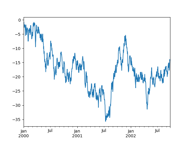
14.13. 绘图 ¶

详情请查看 Plotting:

>>> ts = pd.Series(np.random.randn(1000), index=pd.date_range('1/1/2000', periods=1000))
>>> ts = ts.cumsum()
>>> ts.plot()
    <matplotlib.axes._subplots.AxesSubplot at 0x7ff2ab2af550>

图一

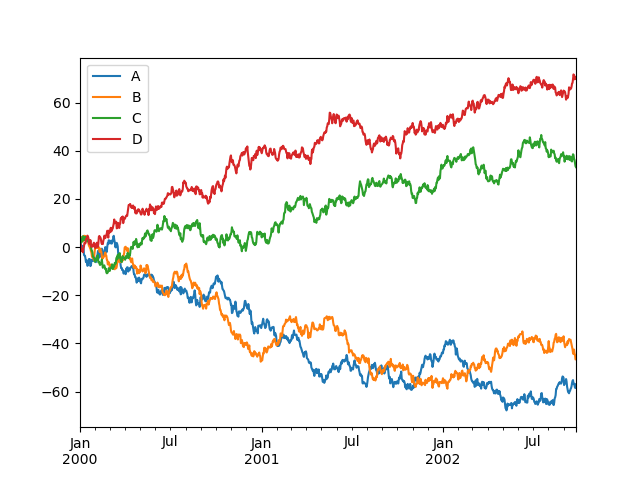
在DataFrame中，plot()可以绘制所有带有标签的列:

>>> df = pd.DataFrame(np.random.randn(1000, 4), index=ts.index,
                      columns=['A', 'B', 'C', 'D'])
>>> df = df.cumsum()
>>> plt.figure(); df.plot(); plt.legend(loc='best')
    <matplotlib.legend.Legend at 0x7ff29c8163d0>

图二

14.14. 获取数据写入导出 ¶

写入csv文件:
```
>>> df.to_csv('foo.csv')
```

读取csv文件:

>>> pd.read_csv('foo.csv')
         Unnamed: 0          A          B         C          D
  2000-01-01   0.266457  -0.399641 -0.219582   1.186860
  2000-01-02  -1.170732  -0.345873  1.653061  -0.282953
  2000-01-03  -1.734933   0.530468  2.060811  -0.515536
  2000-01-04  -1.555121   1.452620  0.239859  -1.156896
  2000-01-05   0.578117   0.511371  0.103552  -2.428202
  2000-01-06   0.478344   0.449933 -0.741620  -1.962409
  2000-01-07   1.235339  -0.091757 -1.543861  -1.084753
    ..          ...        ...        ...       ...        ...
2002-09-20 -10.628548  -9.153563 -7.883146  28.313940
2002-09-21 -10.390377  -8.727491 -6.399645  30.914107
2002-09-22  -8.985362  -8.485624 -4.669462  31.367740
2002-09-23  -9.558560  -8.781216 -4.499815  30.518439
2002-09-24  -9.902058  -9.340490 -4.386639  30.105593
2002-09-25 -10.216020  -9.480682 -3.933802  29.758560
2002-09-26 -11.856774 -10.671012 -3.216025  29.369368

    [1000 rows x 5 columns]

HDF5

HDFStores

1.写入HDF5 Store:

>>> df.to_hdf('foo.h5','df')

2.从HDF5 Store读取:

>>> pd.read_hdf('foo.h5','df')
                        A          B         C          D
    2000-01-01   0.266457  -0.399641 -0.219582   1.186860
    2000-01-02  -1.170732  -0.345873  1.653061  -0.282953
    2000-01-03  -1.734933   0.530468  2.060811  -0.515536
    2000-01-04  -1.555121   1.452620  0.239859  -1.156896
    2000-01-05   0.578117   0.511371  0.103552  -2.428202
    2000-01-06   0.478344   0.449933 -0.741620  -1.962409
    2000-01-07   1.235339  -0.091757 -1.543861  -1.084753
    ...               ...        ...       ...        ...
    2002-09-20 -10.628548  -9.153563 -7.883146  28.313940
    2002-09-21 -10.390377  -8.727491 -6.399645  30.914107
    2002-09-22  -8.985362  -8.485624 -4.669462  31.367740
    2002-09-23  -9.558560  -8.781216 -4.499815  30.518439
    2002-09-24  -9.902058  -9.340490 -4.386639  30.105593
    2002-09-25 -10.216020  -9.480682 -3.933802  29.758560
    2002-09-26 -11.856774 -10.671012 -3.216025  29.369368

    [1000 rows x 4 columns]

Excel

MS Excel

1.写入excel文件:

>>> df.to_excel('foo.xlsx', sheet_name='Sheet1')

2.从excel文件读取:

>>> pd.read_excel('foo.xlsx', 'Sheet1', index_col=None, na_values=['NA'])
                        A          B         C          D
    2000-01-01   0.266457  -0.399641 -0.219582   1.186860
    2000-01-02  -1.170732  -0.345873  1.653061  -0.282953
    2000-01-03  -1.734933   0.530468  2.060811  -0.515536
    2000-01-04  -1.555121   1.452620  0.239859  -1.156896
    2000-01-05   0.578117   0.511371  0.103552  -2.428202
    2000-01-06   0.478344   0.449933 -0.741620  -1.962409
    2000-01-07   1.235339  -0.091757 -1.543861  -1.084753
    ...               ...        ...       ...        ...
    2002-09-20 -10.628548  -9.153563 -7.883146  28.313940
    2002-09-21 -10.390377  -8.727491 -6.399645  30.914107
    2002-09-22  -8.985362  -8.485624 -4.669462  31.367740
    2002-09-23  -9.558560  -8.781216 -4.499815  30.518439
    2002-09-24  -9.902058  -9.340490 -4.386639  30.105593
    2002-09-25 -10.216020  -9.480682 -3.933802  29.758560
    2002-09-26 -11.856774 -10.671012 -3.216025  29.369368

    [1000 rows x 4 columns]

14.15. 小陷阱 ¶

如果你操作时遇到了如下异常:

>>> if pd.Series([False, True, False]):
    ...     print("I was true")
    ...
    Traceback (most recent call last):
    File "<stdin>", line 1, in <module>
      File "/usr/lib64/python2.7/site-packages/pandas/core/generic.py", line 730, in __nonzero__
        .format(self.__class__.__name__))
    ValueError: The truth value of a Series is ambiguous. Use a.empty, a.bool(), a.item(), a.any() or a.all().

请查看 Comparisons 来处理异常查看 Gotchas 也可以

14.16. pandas实战 ¶

***